Co-ordinate Transformations

by John P Scott

Co-ordinate Transformations

Introduction

Translation

Scaling

Rotation

Multiple transformations

Matrix representation of co-ordinates and transformations

Exercises

Introduction

We have now seen that to effectively display real world data on a display we need efficient rendering algorithms with the ability to clip the data to a region on the display and also to map the real world co-ordinate system onto the display co-ordinate system. There is also a need to manipulate the real world data to alter the way we see it on the display. We may want to move an object around the display, rotating it and altering its size. To perform these actions require transformations other than the Window - Viewport transformation we considered earlier.

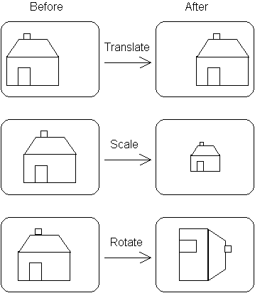
For most applications we only require three basic transformations, and these are demonstrated in Figure 1.

Demonstration of basic transformations

Figure 1.
By combining transformations it is possible to manipulate the displayed image in many ways.

In fact the Window - Viewport transformation we discussed previously is made up of three basic transformations performed one after the other. We will see how to do this later.

Translation

Translation causes the co-ordinates of an object to be altered such that the points all move an equal distance horizontally and/or vertically. Figure 2 gives an example of the effect of translation.

Demonstration of translation

Figure 2.
The amount of translation is given by an offset co-ordinate (tx,ty). The transformed co-ordinate (x',y') is given by:

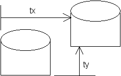
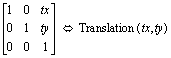
                x' = x + tx
                y' = y + ty

As you can see the calculation is minimal, and you might expect that this is the optimal method.

However, we will see later that this formulation is far from ideal in a real situation.

Scaling

Scaling causes the size of the object to be altered. This may be by different factors in X and Y.

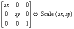
e.g. double the height and half the width. Figure 3 gives an example of the effect of scaling.

Demonstration of scaling

Figure 3.
The amount of scaling is given by a pair of scale factors (sx,sy). The transformed co-ordinate (x',y') is given by:

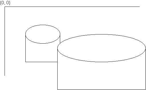
                x' = x * sx
                y' = y * sy

This calculation involves multiplication, but is very simple, and you might expect that this too is the optimal method. Again, this formulation is far from ideal in a real situation.

Rotation

Rotation causes the object to move as if it was pivoting around the origin. The amount of rotation is specified by an angle (A). (Note that angles in Pascal are specified in Radians and if you want to use degrees you need to divide by 180 and multiply by PI. Figure 4 shows the effect of rotation.

Demonstration of Rotation

Figure 3.
The calculation for the transformation in this case is not as straightforward. The transformed co-ordinate is given by:

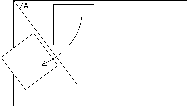
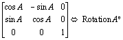
                x' = x * cos(A) - y * sin(A)
                y' = x * sin(A) + y * cos(A)

This transformation not only requires real arithmetic, but it also require trigonometric functions. There is no alternative to using trigonometric functions in this case, but it may be made more efficient by using function tables for sine and cosine.

Multiple transformations

An example of a multiple transformation is a Window Viewport transformation. The first transformation is a translation by (-WXMin, -WYMin), which moves the Window so that it sits on the origin. The second transformation is a scale by

. For an isometric transformation the scale would use equal scaling based on the smaller of the two scales given. This scales the Window to the size of the Viewport. The final transformation is a translating by (VXMin,VYMin) which moves the Viewport to its correct position.

The combined effect of the three transformations is the same as the formula given in the section above.

However, in general terms it may be necessary to perform an arbitrary set of transformations on an image. This would mean having to perform a whole sequence of calculations on each point.

This is not very efficient. A more efficient method would allow any number of transformations to be combined into a single composite transformation, which can then be applied to each point. This is possible if we specify the basic transformations in a different way.

The usual method is to use matrices to represent transformations and co-ordinates. We will discuss this in the next section.

Matrix representation of co-ordinates and transformations

A matrix is a group of numbers organised in a grid of rows and columns. A co-ordinate (x,y) can be represented by a matrix with 3 rows and 1 column as:

Matrix representation of a coordinate
A transformation can also be represented as a matrix, but this time with 3 rows and 3 columns:

Matrix representation of a transformation
The transformation is represented mathematically by the multiplication of the transformation matrix by the co-ordinate matrix. The result is a 3 rows by 1 column matrix which represents the transformed point. The resulting matrix is:

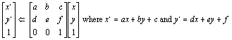
Matrix representation of a transformed coordinate
The three basic transformations are represented by the following transformation matrices:

Matrix representation of translation
Matrix representation of scaling
Matrix representation of rotation
At first it may seem that the effect of using transformation matrices is to complicate the calculation process for the benefit of making the calculation the same for each kind of transformation. However, matrix algebra is very similar to arithmetic algebra. e.g.

Using the matrix approach, if you need to apply transformation T1 to all your data co-ordinates, and then transformation T2 you can combine the two transformations into a single composite matrix and then apply the combined transformation to all the points in one pass. e.g.

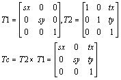
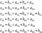
Matrix representation of a combined transformation
The mathematical formulation for multiplying two transformations is:

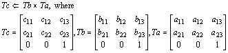
Matrix representation of a composite transformation
giving:

Calculation of a composite transformation
As you can see, the calculation is straightforward, and easy to automate, but there are a lot of calculations. However, these calculations only need to be performed once and then the composite transformation matrix can be applied to all the data points. Figure 5 gives the code for handling matrix representation of co-ordinates and transformations.

TYPE
  TCoordinate = ARRAY [0 .. 2] OF Real;
  TTransformation = ARRAY [0 .. 2, 0 .. 2] OF Real;
CONST
  Identity: TTransformation
        = ((1,0,0),(0,1,0),(0,0,1));
PROCEDURE TransformPoint
     (VAR P: TCoordinate; T: TTransformation);
VAR
  I, J: Integer;
  Temp: TCoordinate;
BEGIN
FOR I := 0 TO 2 DO
  BEGIN
  Temp[I] := 0;
  FOR J := 0 TO 2 DO
     Temp[I] := Temp[I] + T[I,J] * P[J];
  END;
P := Temp
END;
PROCEDURE ComposeTransformation
     (VAR T3: TTransformation;
      T2, T1: TTransformation);
VAR I, J, K: Integer;
BEGIN
FOR I := 0 TO 2 DO
  FOR J := 0 TO 2 DO
    BEGIN
    T3[I,J] := 0;
    FOR K := 0 TO 2 DO
       T3[I,J] := T3[I,J] + T2[I,K] * T1[K,J]
    END
END;
PROCEDURE Translate(TX, TY: Real;
                                                  VAR T: TTransformation);
BEGIN
T := Identity;
T[1,3] := TX;
T[2,3] := TY
END;
PROCEDURE Scale(SX, SY: Real; VAR T: TTransformation);
BEGIN
T := Identity;
T[1,1] := SX;
T[2,2] := SY
END;
PROCEDURE Rotate(A: Real; VAR T: TTransformation);
BEGIN
T := Identity;
T[1,1] := Cos(A);
T[2,1] := Sin(A);
T[1,2] := -T[2,1];
T[2,2] := T[1,1]
END;

Figure 5
Note that the code in Figure 5 does not use the long hand formulation but uses an iterative method based on matrix algebra. This is slightly less efficient for simple applications which only use combinations of the three basic transformations, but some applications require transformations where the bottom row of the transformation matrix is not (0, 0, 1) and so a complete formulation of matrix multiplication is required. Such transformations are beyond the scope of this basic text, but later work on three dimensional graphics will introduce the concepts when dealing with perspective.

Exercises

1. Incorporate the code from Figure 5 into a unit. Use your unit to develop a test program to show the effects of transformations, and combinations of transformations on the display of a simple object.

2. Rewrite the Window - Viewport Transformation program to make use of the transformation unit from exercise 1 above. You will need to express a Window - Viewport transformation as a sequence of basic transformations as described earlier in this section.

Copyright (C) 1995

JPS Graphics, *******************
All rights reserved

Comments to author: *****************